The Statistics Behind the 100-Year Flood
Introduction
In 2013, Colorado experienced a flood that wiped out homes, bridges, and infrastructure. The storm that caused the flooding was brought from the Gulf of Mexico. The Rocky Mountains stalled the mass of tropical rain, but when the storm passed it flooded Colorado. It was devastating to Colorado since the state was, and still is unprepared for tropical rain. The flood is referred to as the “100-Year Flood”. Multiple interpretations of the name may come to mind such as, “a flood that lasts for 100 years”, or “a flood that happens once every 100 years”. This essay will interpret the correct meaning and probability associated with the term “100-Year Flood”.
Determining a Flood
To understand the correct meaning of “100-Year Flood” we first must define streamflow. Streamflow is the volume of water that moves over a point during a fixed period. Stream gauges are set up on the side of rivers to calculate streamflow in cubic feet per second. An area that expects a lot of rain will have a higher streamflow than an area without much rain. Permeability is also an important factor in streamflow. If the land is very permeable, then some water will be absorbed and the streamflow will be less than dry un-permeable ground. Because of these geographical factors, each county has a different streamflow value assigned when categorizing floods (USGS).
The streamflow value assigned when analyzing a flood is determined with a Annual Exceedance Probability (AEP). In other words, a streamflow threshold is determined by the probability the streamflow will exceed at any given year. The AEP for a “100-Year Flood” is 1%. So, the 1% AEP is what determines the streamflow value assigned for a flood to be titled a “100-Year Flood”. The 1% annual probability of exceedance remains the same, but the streamflow is adjusted from county to county in order to maintain the 1% AEP.
To recap, the streamflow that is determined to be considered a “100-Year Flood” is calculated based on which streamflow has a 1% chance of occurring (or exceededing) annually (USGS).
Interpretation of Probability
Now that we know how a flood qualifies as a “100-Year Flood”, we can interpret its meaning more clearly. To be precise, there is a 1% chance in any given year for a flood to be equal to or greater than that county’s given streamflow threshold.
Take Colorado’s 2013 flood as an example. The streamflow corresponding with a 1% AEP in Colorado counties was approximately 5,000 cubic feet per second (CCC). This streamflow value was assigned because, for any given year, there is a 1% chance of a flood with a streamflow of 5,000 cubic feet or more. Since the 2013 streamflow exceeded 5,000 cubic feet the flood was considered a “100-Year Flood”.
The interval of time and probabilities associated are often misinterpreted because of what the “100-Year Flood” title implies. Many people may interpret it as; “there are 100 years between each flood that equals or exceeds the given streamflow”. Instead, 100 years is the estimate of the long-term average recurrence interval. This is the long-term average estimate since each year is independent of one another. So, each year there is a 1% probability of a “100-Year Flood” occurring, no matter what has happened in the other years. For that reason, a probability assigned to the 100-year interval of time would be an incorrect interpretation.
The AEP of 1% for a “100-year flood” is used because it gives an idea of the magnitude of the flood. Since different geographies handle the same streamflow better or worse, determining a flood’s rarity and magnitude on the streamflow alone is not effective. The AEP gives us more information about the flood’s likelihood without needing geography context.
The same applies to other flood magnitudes that occur more or less often. A “10-Year Flood” has a 10% AEP and a “500-Year Flood” has a .2% AEP. The likelihoods of these floods are different so they have different probabilities assigned to them. The bigger floods are less likely to occur; similarly, the smaller ones are more likely to occur. In other words, flood magnitude is positively correlated to recurring intervals. For example, for a flood to be deemed a “500-Year Flood,” the streamflow must be equal to or greater than the threshold assigned for that .2% AEP and is therefore more severe than the 10 or 100 year floods.
The table below shows the AEP for floods with different recurrence intervals.
| Recurring Interval (years) | Annual Exceedance Probability (AEP) |
|---|---|
| 2 | 50% |
| 5 | 20% |
| 10 | 10% |
| 50 | 2% |
| 100 | 1% |
| 500 | 0.2% |
| 1000 | 0.1% |
(USGS)
The first row can be interpreted as floods with magnitudes that are reached approximately every two years, have a 50% chance of occurring in any given year. For example, the year 2000 would have a 50% AEP, then if a flood (above the “2-Year Flood” AEP assigned streamflow) occurred, the year 2001 would still have a 50% AEP. The recurring interval is simply the long-term estimate of an interval and is used to give a general idea of how often the event occurs.
In order to have a correct interpretation of the AEP, the probability must be associated with a one-year time frame.
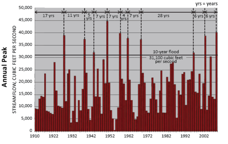
The graph above demonstrates how often a “10-Year Flood” occurs in the Embarras River in Illinois.
(USGS1)
Each year, the Embarras River has a 10% probability of exceeding 31,100 cubic feet per second, regardless of what occurred in prior years.
These Annual Exceedance Probabilities are assigned using a frequentist methodology. The streamflow for a given AEP is determined by analyzing historical streamflow data. Then the likelihood of floods is calculated for various magnitudes based on the observed frequencies of past events and simulations. Specifically, flood probabilities can be calculated using the Binomial distribution. The Binomial distribution can be used since there are two possible outcomes; the flood occurring and the flood not occurring.
The freuentist binomial approach also allows us to simulate many floods which assigns a hypothetical relative frequency. A simple example of a hypothetical relative frequency is simulating flipping a fair coin. If you simulate flipping a fair coin 1,000 times, the probability of heads will be close to 50%. The alternative frequentist approach is the finite frequency. A finite frequency assigns probability using only the data on hand. So if you flip a fair coin 10 times and it lands on heads 6 times, the probability of heads is 60%. The hypothetical relative frequency is used for flooding estimation since we do not have to rely solely on the observed data. Relying on observed data for rare floods such as a “500-Year Flood” will not produce results that reflect the big picture since the sample size of infrequent floods is limited.
The binomial equation can be used to calculate the probability of a flood with a 1% AEP (a “100-Year flood”) happening exactly one time in the span of 100-Years:
\[ {n \choose k}(n k)p^k (1-p)^{n-k} \]
\[ {100 \choose 1} .01^1 (1-0.01)^{99} = 0.37 \]
From the binomial equation, we can interpret .37 as; there is a 37% chance of a “100-Year flood” occurring once within 100 years. But the 100-year flood has 1% AEP or 1/100 AEP. So the fact that there is only a 37% chance of the flood occurring once over 100 years makes the name “100-Year Flood” lead to misinterpretation of the frequency of the flood.
The probability of exactly two, 100-year floods within a 100-year interval is:
\[ 1-(1-.01)^{100}= 0.634 \]
The same logic can be applied to finding the probability of 2,3, or 4 “100-Year Floods” occurring in 100-years:
| Number of Floods in a Year | Annual Exceedance Probability (AEP) |
|---|---|
| 0 | 36.6% |
| 1 | 37% |
| 2 | 18.5% |
| 3 | 6.1% |
| 4 | 1.4% |
| At least 1 | 63.4% |
The probability of a flood occurring in a given year can also change when a flood has already happened that same year. Conveniently, the binomial distribution can be used to calculate conditional probabilities.
The code below gives the probability equation to calculate exactly two “100-Year Floods” occur in 100 years given that at least one occurs:
dbinom(x = 2, size = 100, prob = 0.01)/pbinom(q = 0, size = 100, prob = 0.01, lower.tail = FALSE)[1] 0.2915998The probability of two “100-Year Floods” within 100 years given that at least one has already occurred is 29% (Ladson).
Assigning probabilities using the frequentist method seems reliable for flood predictions. The name of the flood is determined in a broad, big-picture sense, so the frequentist method is effective in assigning a probability to correspond with a general name.
Counterarguement to Frequentist Approach
Some would argue that the Bayesian method is more effective. Even though the frequentist method is effective for predictions, there are arguments that the Bayesian methodology should be used for flood analysis.
The Bayesian forecasting method calculates probabilities differently, and some claim to be more accurate (Han). However, using the Bayesian model changes the probabilities and interpretations. An argument for the Bayesian approach is the interpretation of probability may not be as confusing as the frequentists.
The Bayesian method gives a probability of uncertainty. This can make the interpretation of a flood’s occurrence more straightforward than the frequentist’s. However, the counterargument is flooding should be measured by the frequency of the phenomenon rather than our degree of belief. Therefore the frequentist approach is most relevant to floods. If a Bayesian claims their approach is more accurate, one can make the argument that the frequentist approach will become more accurate as more conditions are used. A frequentist can have more confidence in the probability as more specifications are made. Using time of year, cloud density, and other factors that can influence the chance of a flood, and make the probability more confident.
Conclusion
Once the frequentist approach is spelled out, the 2013 Colorado flood’s probabilities associated with it can be correctly interpreted. From first glance it is easy to draw the wrong conclusion about frequency of floods so, maybe these floods need a new name. However it is not the fault of the frequentist methodology that these probabilities are misinterpreted. The frequentist approach gives us a stronger understanding of the frequency of extreme floods and the ability to understand when the next one could occur.
Citations
CCC. “Colorado Flood 2013.” Colorado Flood 2013 Storm Page - Runoff, Colorado State University, coflood2013.colostate.edu/runoff.html. Accessed 8 Oct. 2023.
Han, Shasha. “Bayesian flood forecasting methods: A review” ScienceDirect, https://www.sciencedirect.com/science/article/abs/pii/S0022169417304031
Ladson, Tony. “Flood Binomial Distribution” tonyladson, https://tonyladson.wordpress.com/2019/09/12/1-flood-binomial-distribution-conditional-probabilities/
USGS. “The 100-Year Flood .” United States Geological Survey, www.usgs.gov/special-topics/water-science-school/science/100-year-flood#overview. Accessed 8 Oct. 2023.
USGS1. “Large Variability in Yearly Peak Streamflow Affects Flood Designations.” United States Geological Survey, www.usgs.gov/media/images/large-variability-yearly-peak-streamflow-affects-flood-designations. Accessed 8 Oct. 2023.