Global Wage Prediction Model
This page is still in progress!
Introduction
As someone who has considered pursuing a higher level of education, I often wonder how much this will enhance my work earnings, not only in the United States, but across the world. For this project I am exploring the strength of the linear relationship between wages and age, sex, country, and level of education. I created a Multiple Regression Model to predict how my income will change if I move to another continent, and how my income in those different continents shifts when my education level changes from a bachelor’s to a masters or doctorate. The goal is to be able to recognize how different countries value education by calculating those differences. The predictors are age, sex, country, and level of education, while wage is the response.
The null and alternate hypothesis for the F-statisic are as follows:
Null Hypothesis: There is no statistical association between the predictors and the response
Alternative Hypothesis: There is some statistical association between at least one of the predictors and the response
Data Preparation
The Organisation for Economic Co-operation and Development(OECD) is the data source I retrieved my information from. Countries that are part of the organization have governments committed to democracy and the international market economy. The original data came from Education at a Glance, a source that tracks data on education around the world.
One important variable to understand about my data set is how the predictor, income, is presented. Since this data encompasses all OECD countries, wage levels are calculated by dividing low and high pay. Low pay is the share of workers that earn less than two thirds of median wage while high pay is the share of workers that earn more than one and a half of median wage.
All of my predictor variables are categorical. The sex is a qualitative, nominal variable assigned as male and female. Age is ordinal and is in groups set at 25-34, and 55-64. Education level is also an ordinal and categorical with variables, upper secondary education(equivalent to high school degree in the U.S.), bachelor’s or equivalent education, and master’s, doctoral or equivalent education. One important change I made to the data set was adding a column of continents. Since understanding the data strictly by country there are too many variables, and adding continents made it easier to understand big picture differences. Categorizing by continent also gave me the opportunity to visualize the data neatly.
Exploratory Analysis
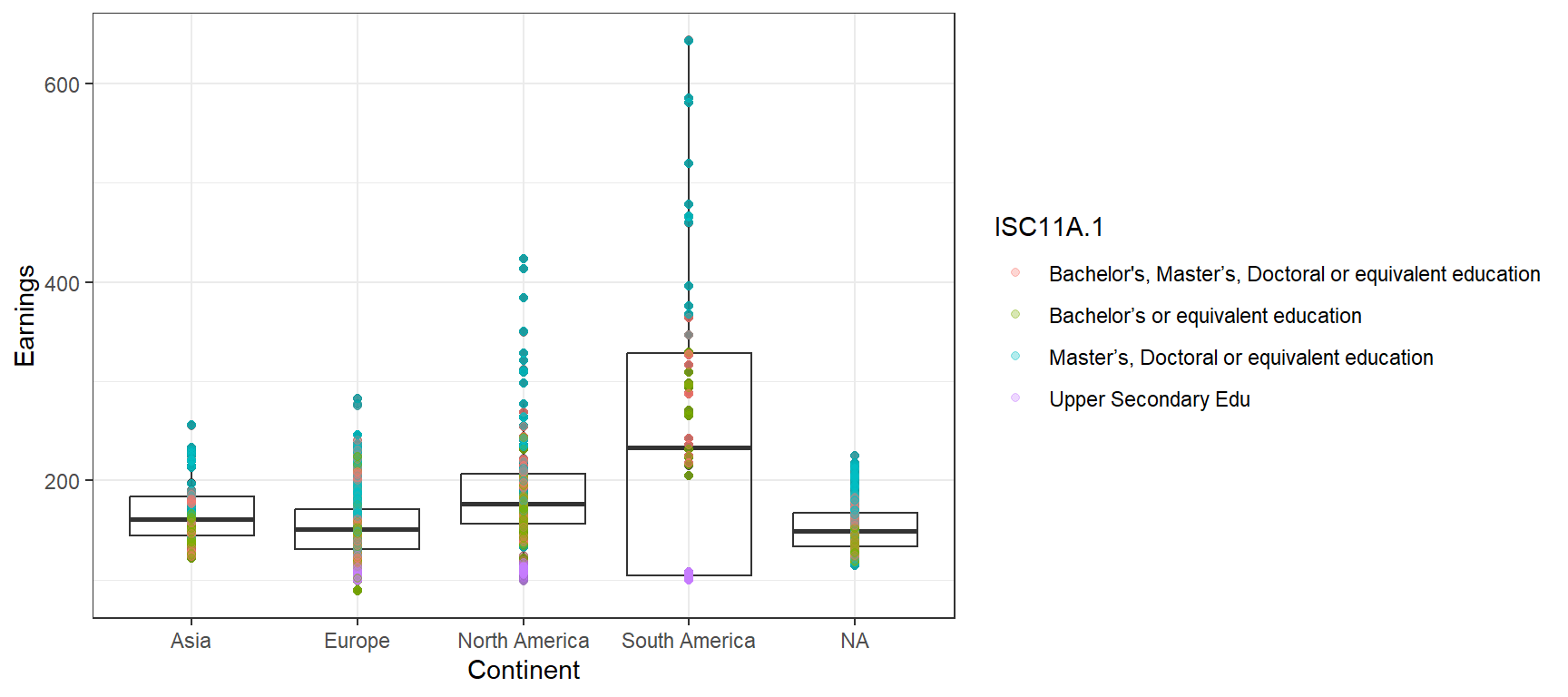
Figure 1
* NA is Oceania and islands
As expected, the higher your level of education is, the higher your earnings are on average. None of the predictors taken from this source are dependent on one another, so there is no double counting within the model. No predictors are correlated with one another, but some are individually correlated with the response.
Model Development
My null hypothesis under the F-statistic is that there is no statistical association between age, level of education, continent and wage. The alternate hypothesis under the F-statistic is there is at least one variable out of age, level of education, and continent with statistical association to wage. My null hypothesis and alternate hypothesis is the same idea as the F-statistic, but instead compares each individual variable rather than at least one.
I split my data where 70% is in the training set, while the other 30% is in the test set. For my model I have the goal of prediction, so the hierarchical rule does not apply, and since we are using a multiple regression model, we do not need to worry about any violation of normality. Since variables are independent, lack co linearity, and do not have any influential outliers, all assumptions have been validated and the final regression model is suitable for prediction.
Using backward step-wise selection I removed variables that did not have as high of p-values than others. This resulted in me taking out levels of education that are equivalent to Middle and Elementary grades in the U.S. One result I was surprised to see was that sex negatively affected the accuracy of the model, so I chose to remove it as well.
The total number of variables that resulted in the lowest Adjusted R-Squared was the model with 7 predictor variables. You can see in the Adjusted R-Squared plot and the Residual sum of squares plot that 7 variables is when the model’s accuracy stops growing.
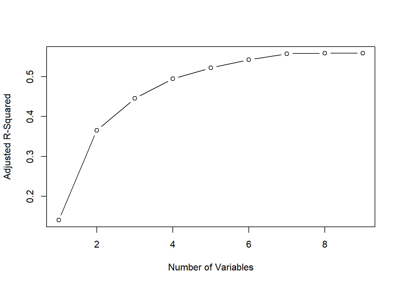
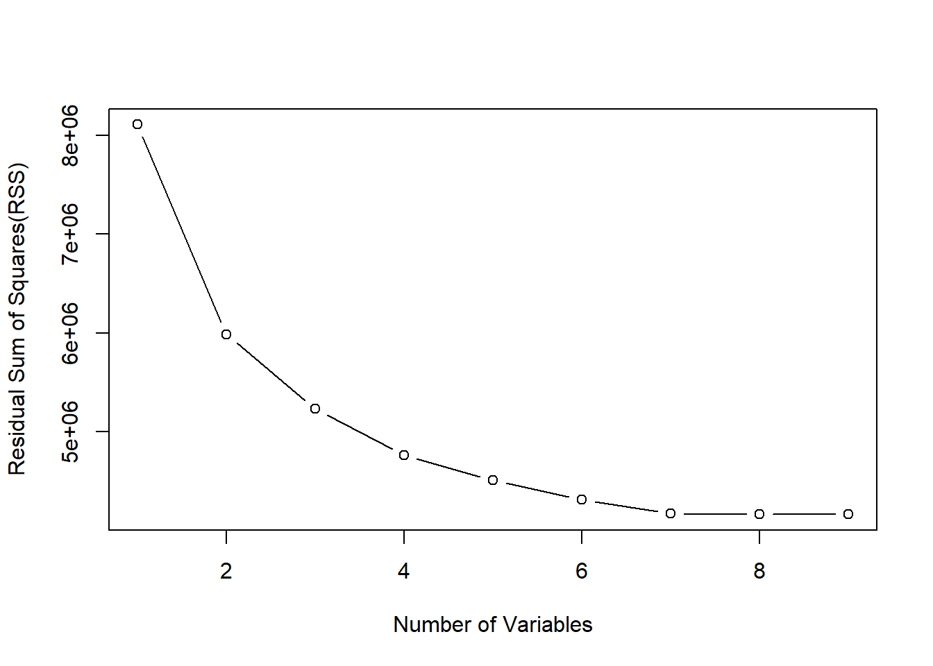
Figure 2, 3
In Figure 2 and 3 the model is taking the 7 best predictors and showing their influence on the accuracy of the model using Adjusted R-Squared and the Residual Sum of Squares.
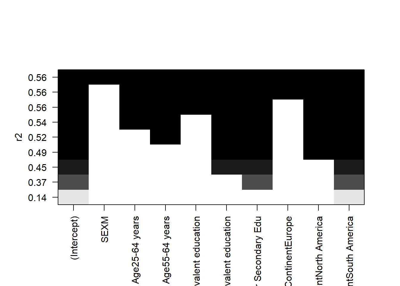
Figure 4
Ultimately the predictors that gave me the most accurate model were age, level of education, and location. You can see the predictor’s significance visually in Figure 4 and quantitatively in the model summary in Figure 5.
Call:
lm(formula = Value ~ Age + ISC11A.1 + Continent, data = educvarstrain)

Residuals:
    Min      1Q  Median      3Q     Max
-109.60  -19.44   -2.74   15.54  325.88

Coefficients:
                                                   Estimate Std. Error t value
(Intercept)                                         149.729      3.382  44.266
Age25-64 years                                       17.761      1.855   9.574
Age55-64 years                                       27.392      1.891  14.486
ISC11A.1Bachelor’s or equivalent education          -19.023      1.963  -9.692
ISC11A.1Master’s, Doctoral or equivalent education   26.366      1.986  13.276
ISC11A.1Upper Secondary Edu                         -81.724      2.763 -29.577
ContinentEurope                                      -6.211      3.120  -1.991
ContinentNorth America                               29.220      3.665   7.973
ContinentSouth America                              114.201      4.470  25.546
                                                   Pr(>|t|)
(Intercept)                                         < 2e-16 ***
Age25-64 years                                      < 2e-16 ***
Age55-64 years                                      < 2e-16 ***
ISC11A.1Bachelor’s or equivalent education          < 2e-16 ***
ISC11A.1Master’s, Doctoral or equivalent education  < 2e-16 ***
ISC11A.1Upper Secondary Edu                         < 2e-16 ***
ContinentEurope                                      0.0466 *
ContinentNorth America                             2.48e-15 ***
ContinentSouth America                              < 2e-16 ***
---
Signif. codes:  0 '***' 0.001 '**' 0.01 '*' 0.05 '.' 0.1 ' ' 1

Residual standard error: 35.61 on 2156 degrees of freedom
  (1085 observations deleted due to missingness)
Multiple R-squared:  0.5664,    Adjusted R-squared:  0.5648
F-statistic:   352 on 8 and 2156 DF,  p-value: < 2.2e-16
Figure 5
Model Assessment
The result from the summary of my model in Figure 5 includes a F-statistic p-value of \< 2.2e-16 which immediately indicates that there is some statistical association between at least one of the predictors and the response. I reject the null hypothesis in favor of the alternate. The same applies for each individual predictor variable. After performing backward-stepwise selection, each variable has some statistical association with wage. The adjusted R-squared is lower than ideal at 0.5855 meaning that 59% of variation of age, education, and continent, can be explained by the linear association with wage. This result is to be expected since we are predicting for 5 continents. When we eventually focus on one specific area, the result is more accurate since there is less variability in the data.
The residual standard error is 38.73 on 1500 degrees of freedom, meaning we can expect our prediction to be off by an average 38.73 percentage points. This error is not bad, in the context of the problem, since we are evaluating values ranging from 88% to 650%.
To identify outliers in the model, we refer to the Scale-Location plot in Figure 6.
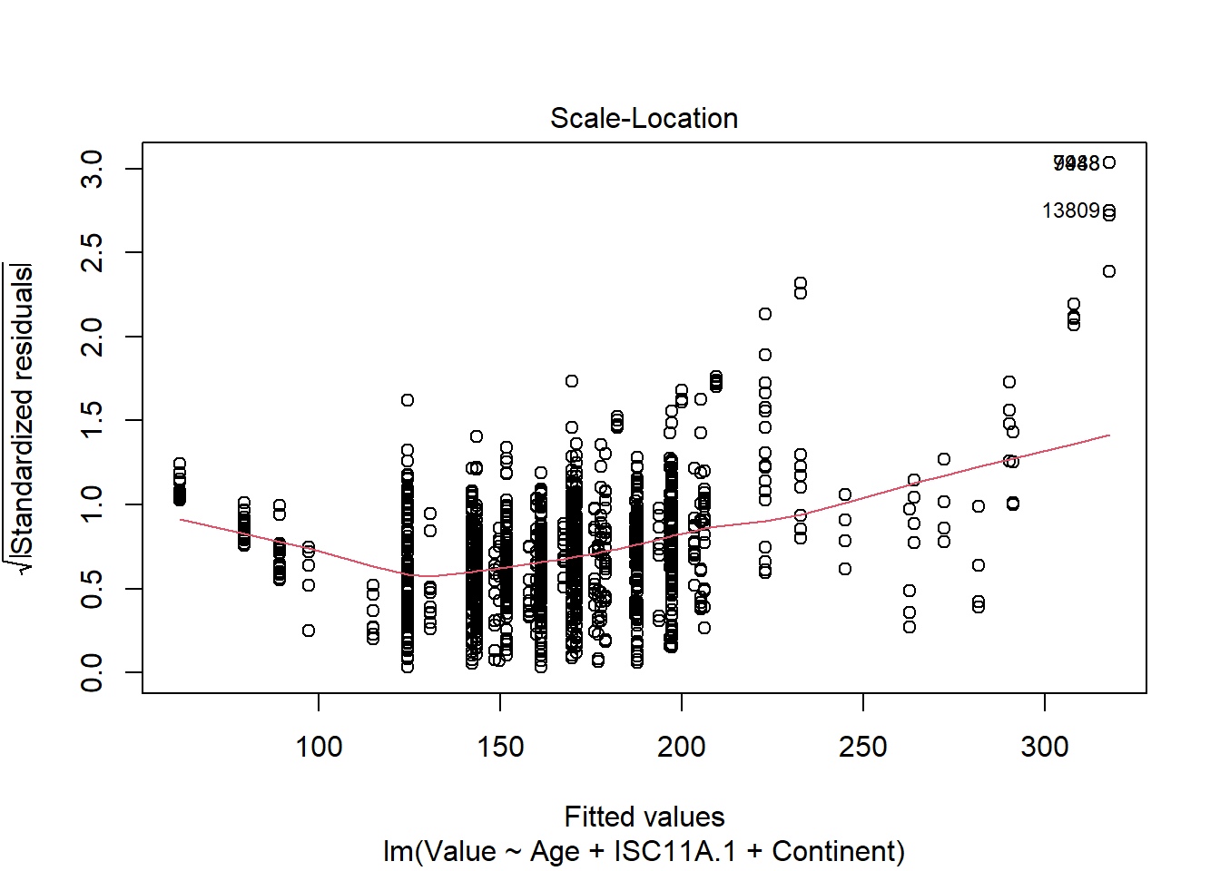
Figure 6
The outliers in this model are both from Chile. These two points have master’s and doctoral as their level of education with age 55-64 years, where the only difference is sex. The first is data point 11861, which is the farthest outlier, is female. Slightly below is data point 13809 which is the same in all variables except the sex is male. The earnings were 644% and 586%. When viewing the highest wages of the data set as a whole, these points are some of the highest. In fact, all the highest wages are in Chile. Upon further research I can now see that Chile has an extremely high poverty rate, and their income distribution is large, so it would make sense that a master’s or doctorate is valued the most in terms of earnings in Chile. Since these outliers do not lie within Cook’s Distance they are not highly influential points, and I see no reason to remove them.
The calculated root mean squared error(RMSE) is 47%. This was found by using the test set to calculate the difference between the predicted income vs actual income, then squaring the difference, taking the mean, and then finally taking the square root.
Since I want to predict what my own potential salary could be if I went from a bachelor’s to a master’s, or doctorate, I created a separate model for North America, South America, Europe, and Asia. This will allow me to see which continents value that extra level of education the most.
North America
Call:
lm(formula = Value ~ ISC11A.1 + Age + SEX, data = na_datatrain)

Residuals:
     Min       1Q   Median       3Q      Max
-113.052  -20.040   -4.606   16.807  176.363

Coefficients:
                                                   Estimate Std. Error t value
(Intercept)                                         163.629      5.734  28.536
ISC11A.1Bachelor’s or equivalent education          -12.246      5.774  -2.121
ISC11A.1Master’s, Doctoral or equivalent education   56.115      6.120   9.169
ISC11A.1Upper Secondary Edu                         -77.700      9.231  -8.417
Age25-64 years                                       29.204      5.594   5.221
Age55-64 years                                       22.856      5.966   3.831
SEXM                                                  4.760      4.673   1.019
                                                   Pr(>|t|)
(Intercept)                                         < 2e-16 ***
ISC11A.1Bachelor’s or equivalent education         0.034772 *
ISC11A.1Master’s, Doctoral or equivalent education  < 2e-16 ***
ISC11A.1Upper Secondary Edu                        1.77e-15 ***
Age25-64 years                                     3.40e-07 ***
Age55-64 years                                     0.000156 ***
SEXM                                               0.309213
---
Signif. codes:  0 '***' 0.001 '**' 0.01 '*' 0.05 '.' 0.1 ' ' 1

Residual standard error: 40.16 on 291 degrees of freedom
  (29 observations deleted due to missingness)
Multiple R-squared:  0.4918,    Adjusted R-squared:  0.4813
F-statistic: 46.93 on 6 and 291 DF,  p-value: < 2.2e-16
Figure 7
* see Data Preparation to interpret income percent
Figure 7 has an Adjusted R-squared 48%, meaning 48% of variation in sex, age, and education can be explained by its linear association with earnings in North America. This score is the lowest of the continents because of the level of variation in the data, which you can see when predicting how large the earnings interval is.
I am 95% confident that if I, a female, worked in North America and am between 25-34 years old with a bachelor’s or equivalent, my income would be between 57% and 249%. This is a huge range of values that your income could be! The 57% is the lowest wage percentage you will see, meaning if you get a Bachelors in North America you have a fairly high chance of getting an income on the lower side. This makes me believe that the countries do not value the Bachelor’s degree as much as other countries in the world. However if everything were the same, except my level of education was instead a Master’s or Doctoral equivalent, my income would be between 123% and 315%.
Achieving a high level of education such as a masters or doctoral definitely gives someone better odds of earning a higher wage. The difference of expected wage between the bachelors and masters or doctorate, is a 66% increase in earnings.
South America
Call:
lm(formula = Value ~ ISC11A.1 + SEX + Age, data = sa_datatrain)

Residuals:
    Min      1Q  Median      3Q     Max
-72.122 -13.874  -2.105  11.361 128.005

Coefficients:
                                                   Estimate Std. Error t value
(Intercept)                                         244.633      8.995  27.198
ISC11A.1Bachelor’s or equivalent education          -21.064     10.162  -2.073
ISC11A.1Master’s, Doctoral or equivalent education  180.444     10.128  17.816
ISC11A.1Upper Secondary Edu                        -186.322      9.020 -20.657
SEXM                                                 -6.545      6.667  -0.982
Age25-64 years                                       49.217      8.144   6.043
Age55-64 years                                       90.486      8.166  11.081
                                                   Pr(>|t|)
(Intercept)                                         < 2e-16 ***
ISC11A.1Bachelor’s or equivalent education           0.0404 *
ISC11A.1Master’s, Doctoral or equivalent education  < 2e-16 ***
ISC11A.1Upper Secondary Edu                         < 2e-16 ***
SEXM                                                 0.3283
Age25-64 years                                     1.88e-08 ***
Age55-64 years                                      < 2e-16 ***
---
Signif. codes:  0 '***' 0.001 '**' 0.01 '*' 0.05 '.' 0.1 ' ' 1

Residual standard error: 36.71 on 116 degrees of freedom
  (154 observations deleted due to missingness)
Multiple R-squared:  0.9372,    Adjusted R-squared:  0.934
F-statistic: 288.7 on 6 and 116 DF,  p-value: < 2.2e-16
Figure 8
The adjusted R-squared of Figure 8 is 94%, the highest linear association of all the models!
I am 95% confident that if I worked in South America and am between 25-34 years old with a bachelor’s or equivalent, my income would be between 156% and 319%. This is a major increase in earnings compared to North America. If the predictors remained constant, except my level of education was instead a Master’s or Doctoral equivalent, my income would be between 358% and 522%.
A higher level of education such as a masters or doctoral practically guarantees a higher wage. This makes intuitive sense because South America, a less developed country than the rest in comparison, has a high demand for people with higher levels of education. Having a bachelors versus masters or doctorate results in an average of 202% earnings increase.
Europe
Call:
lm(formula = Value ~ ISC11A.1 + SEX + Age, data = eur_datatrain)

Residuals:
    Min      1Q  Median      3Q     Max
-51.844 -14.697  -2.457  11.027 117.898

Coefficients:
                                                   Estimate Std. Error t value
(Intercept)                                        146.4406     1.3052 112.201
ISC11A.1Bachelor’s or equivalent education         -18.5142     1.3769 -13.447
ISC11A.1Master’s, Doctoral or equivalent education  12.8424     1.3442   9.554
ISC11A.1Upper Secondary Edu                        -55.5191     1.9745 -28.118
SEXM                                                 0.5341     1.0677   0.500
Age25-64 years                                      13.8024     1.3007  10.612
Age55-64 years                                      25.0174     1.2987  19.263
                                                   Pr(>|t|)
(Intercept)                                          <2e-16 ***
ISC11A.1Bachelor’s or equivalent education           <2e-16 ***
ISC11A.1Master’s, Doctoral or equivalent education   <2e-16 ***
ISC11A.1Upper Secondary Edu                          <2e-16 ***
SEXM                                                  0.617
Age25-64 years                                       <2e-16 ***
Age55-64 years                                       <2e-16 ***
---
Signif. codes:  0 '***' 0.001 '**' 0.01 '*' 0.05 '.' 0.1 ' ' 1

Residual standard error: 21.43 on 1606 degrees of freedom
  (276 observations deleted due to missingness)
Multiple R-squared:  0.5221,    Adjusted R-squared:  0.5203
F-statistic: 292.4 on 6 and 1606 DF,  p-value: < 2.2e-16
Figure 9
Figure 9 has an adjusted R-squared of 57%, a lower association than we would prefer but still relevant.
I am 95% confident that if I worked in Europe and am between 25-34 years old with a bachelor’s or equivalent, my income would be between 86% and 172%. This interval does not guarantee as good of a wage with a bachelors than South America does. However if everything were the same except my level of education was instead a master’s or doctoral, my income would be between 118% and 204%.
Obtaining a high level of education such as a master’s or doctoral definitely gives someone better odds of earning a higher wage, but does not guarantee it. The difference of expected wage between the bachelors and masters or doctorate, is a 32% increase in earnings.
Asia
Call:
lm(formula = Value ~ ISC11A.1 + SEX + Age, data = asia_datatrain)

Residuals:
    Min      1Q  Median      3Q     Max
-30.529 -13.385  -4.582  10.728  41.269

Coefficients:
                                                   Estimate Std. Error t value
(Intercept)                                         142.634      3.640  39.188
ISC11A.1Bachelor’s or equivalent education          -11.406      3.537  -3.225
ISC11A.1Master’s, Doctoral or equivalent education   38.537      3.540  10.885
SEXM                                                 -8.515      2.866  -2.971
Age25-64 years                                       24.776      3.572   6.937
Age55-64 years                                       34.128      3.437   9.931
                                                   Pr(>|t|)
(Intercept)                                         < 2e-16 ***
ISC11A.1Bachelor’s or equivalent education          0.00155 **
ISC11A.1Master’s, Doctoral or equivalent education  < 2e-16 ***
SEXM                                                0.00346 **
Age25-64 years                                     1.19e-10 ***
Age55-64 years                                      < 2e-16 ***
---
Signif. codes:  0 '***' 0.001 '**' 0.01 '*' 0.05 '.' 0.1 ' ' 1

Residual standard error: 17.65 on 147 degrees of freedom
  (73 observations deleted due to missingness)
Multiple R-squared:  0.7129,    Adjusted R-squared:  0.7031
F-statistic:    73 on 5 and 147 DF,  p-value: < 2.2e-16
Figure 10
The adjusted R-Squared in Figure 10 is 76%, meaning there is a strong linear association between the predictors and the response.
I am 95% confident that if I worked in Asia and was between 25-34 years old with a bachelor’s or equivalent, my income would be between 93% and 163%. If everything were the same, except my level of education was a master’s or doctoral equivalent, my income would be between 146% and 216%.
Achieving a high level of education such as a masters or doctoral gives someone much better odds of earning a higher wage. The difference of expected wage between the bachelor’s and master’s or doctorate, is a 53% increase in earnings.
Conclusion
Predicting income on a national level is something my model offers over perhaps a more standard model focused in one area. I wanted to see the big picture on a global scale, and this model encompasses countries whose population totals to about 1.38 billion people. One additional bonus that I did not expect to come out of my model was the fluctuation of the p-value of sex in Figures 7-11. Europe, North America, and South America had higher p-values meaning sex plays less of a role in wages. However Asia had a p-value below .05 meaning, being female vs male plays a major role in a person’s earnings. These models expose a lot about country’s development as well as factors they value in the workforce. These would be ultimately benefit any person who wants to travel and/ or is thinking about pursuing a higher level of education.
Citations
“Chile Overview.” World Bank, <https://www.worldbank.org/en/country/chile/overview>.
“Education and Earnings .” OECD, <https://stats.oecd.org/Index.aspx?DataSetCode=EAG_EARNINGS>.
Appendix
Here is all the code used to obtain the results above.
library(tidyverse)

library(mosaic)

library(knitr)

library(tinytex)

library(leaps)

library(knitr)

knitr::opts_chunk$set(echo = TRUE)

knitr::opts_chunk$set(message = FALSE)

knitr::opts_chunk$set(warning = FALSE)

knitr::opts_chunk$set(out.width = "50%")

educvars <- read.csv("education_earnings.csv")%>%

  subset(select = -ISC11A)%>%

  subset(select = -AGE)%>%

  subset(select = -COUNTRY)%>%

  subset(select = -INDICATOR)%>%

  subset(select = -MEASURE)%>%

  subset(select = -Measure)%>%

  subset(select = -YEAR)%>%

  subset(select = -Year)%>%

  subset(select = -Unit.Code)%>%

  subset(select = -Unit)%>%

  subset(select = -PowerCode.Code)%>%

  subset(select = -PowerCode)%>%

  subset(select = -Flag.Codes)%>%

  subset(select = -Flags)%>%

  subset(select = -Reference.Period.Code)%>%

  subset(select = -Gender)%>%

  subset(select = -Indicator)%>%

  subset(select = -EARN_CATEGORY)%>%

  subset(select = -EARN_CATEGORY.1)%>%

  subset(SEX!="T")%>%

  subset(ISC11A.1 != "Below upper secondary education")%>%

  subset(ISC11A.1 != "Tertiary education")%>%

  subset(ISC11A.1 != "Short-cycle tertiary education")%>%

  subset(ISC11A.1 != "Bachelor's, Master's, Doctoral or equivalent education")%>%

  subset(ISC11A.1 != "Post-secondary non-tertiary education")

educvars$ISC11A.1[educvars$ISC11A.1 == "Upper secondary, post-secondary non-tertiary education and short-cycle tertiary education"]<- "Upper Secondary Edu"

educvars$ISC11A.1[educvars$ISC11A.1 == "Master's, Doctoral or equivalent education"]<- "Master's,Doctoral/equivalent"

north_america<- c("United States", "Canada", "Costa Rica", "Mexico")

south_america<-c("Chile", "Colombia", "Dominican Republic", "Ecuador", "El Salvador","Panama","Paraguay", "Brazil")

europe<- c("Austria", "Belgium", "Czech Republic", "Denmark","Estonia","Finland", "France", "Germany", "Greece","Hungary", "Iceland","Ireland","Italy","Latvia","Lithuania","Luxembourg","Netherlands","Norway", "Poland","Portugal", "Slovakia","Slovenia","Spain","Sweden","Switzerland", "Turkey", "United Kingdom", "Luxembourg")

asia<- c("Israel", "Japan","South Korea", "Singapore","Thailand", "Malaysia", "Cambodia", "Korea", "Türkiye")

attach(educvars)

educvars$Continent[Country %in% north_america]<-"North America"

educvars$Continent[Country %in% europe]<-"Europe"

educvars$Continent[Country %in% south_america]<-"South America"

educvars$Continent[Country %in% asia]<-"Asia"

detach(educvars)

#Seperating Each Data Set by Continent

na_data<-educvars%>%

  subset(Continent == "North America")

sa_data<-educvars%>%

  subset(Continent == "South America")

eur_data<-educvars%>%

  subset(Continent == "Europe")

asia_data<-educvars%>%

  subset(Continent == "Asia")

set.seed(101)

sample <- sample.int(n=nrow(educvars),size=floor(0.7*nrow(educvars)),replace=FALSE)

educvarstrain <- educvars[sample,]

educvarstest <- educvars[-sample,]


summary(educvars)
ggplot(data=educvars,aes(x=Continent,y=Value)) +

  ylab("Earnings")+

  geom_jitter(width=0,height=0.1,alpha=0.3) +

  geom_boxplot(alpha=0)+

  geom_point(alpha=.3, aes(color=ISC11A.1))+

  theme_bw()
choosing<-regsubsets(Value~SEX+Age+ISC11A.1+Continent, data=educvars, nvmax=10, method="backward")

choosing.summary<-summary(choosing)

plot(choosing.summary$rsq, xlab = "Number of Variables", ylab="Adjusted R-Squared", type="b")

plot(choosing.summary$rss, xlab = "Number of Variables", ylab = "Residual Sum of Squares(RSS)", type="b")
#which.max(choosing.summary$adjr2)

plot(choosing, scale = "r2")
model6<-lm(Value~Age+ISC11A.1+Continent, data=educvarstrain)

summary(model6)
plot(model6, which=3)
test_predict1 <- educvarstest %>%

  mutate(prob=predict(model6,newdata=educvarstest,type='response'))

test_predict1 %>%

  summarize(accuracy=sqrt(mean((prob-Value)^2, na.rm=TRUE)))
#using na_data

set.seed(101)

sample <- sample.int(n=nrow(na_data),size=floor(0.7*nrow(na_data)),replace=FALSE)

na_datatrain <- na_data[sample,]

na_datatest <- na_data[-sample,]

model7<-lm(Value~ISC11A.1+Age+SEX, data=na_datatrain)

summary(model7)

#plot(model7)

#predict(model7, newdata=data.frame(SEX="F", Age = "25-34 years", ISC11A.1= "Bachelor’s or equivalent education"), interval="prediction", level=.95)

#predict(model7, newdata=data.frame(SEX="F", Age = "25-34 years", ISC11A.1= "Master's,Doctoral/equivalent"), interval="prediction", level=.95)
#using sa_data

set.seed(101)

sample <- sample.int(n=nrow(sa_data),size=floor(0.7*nrow(sa_data)),replace=FALSE)

sa_datatrain <- sa_data[sample,]

sa_datatest <- sa_data[-sample,]

model8<-lm(Value~ISC11A.1+SEX+Age, data=sa_datatrain)

summary(model8)

#predict(model8, newdata=data.frame(SEX="F", Age = "25-34 years", ISC11A.1="Bachelor's or equivalent education"), interval="prediction", level=.95)

#predict(model8, newdata=data.frame(SEX="F", Age = "25-34 years", ISC11A.1="Master's,Doctoral/equivalent"), interval="prediction", level=.95)
set.seed(101)

sample <- sample.int(n=nrow(eur_data),size=floor(0.7*nrow(eur_data)),replace=FALSE)

eur_datatrain <- eur_data[sample,]

eur_datatest <- eur_data[-sample,]

model9<-lm(Value~ISC11A.1+SEX+Age, data=eur_datatrain)

summary(model9)

#predict(model9, newdata=data.frame(SEX="F", Age = "25-34 years", ISC11A.1="Bachelor's or equivalent education"), interval="prediction", level=.95)

#predict(model9, newdata=data.frame(SEX="F", Age = "25-34 years", ISC11A.1="Master's,Doctoral/equivalent"), interval="prediction", level=.95)
set.seed(101)

sample <- sample.int(n=nrow(asia_data),size=floor(0.7*nrow(asia_data)),replace=FALSE)

asia_datatrain <- asia_data[sample,]

asia_datatest <- asia_data[-sample,]

model10<-lm(Value~ISC11A.1+SEX+Age, data=asia_datatrain)

summary(model10)

#predict(model10, newdata=data.frame(SEX="F", Age = "25-34 years", ISC11A.1="Bachelor's or equivalent education"), interval="prediction", level=.95)

#predict(model10, newdata=data.frame(SEX="F", Age = "25-34 years", ISC11A.1="Master's,Doctoral/equivalent"), interval="prediction", level=.95)